Traditionally, time series data have been thought to consist of four separate components:
Trend - long-term movement up or down, such as general increases in the level of the world’s economy.
Cycle - cyclical fluctuations around the trend line, caused by irregular movements as in a typical business cycle of expansion and contraction.
Seasonality - periodic movement of a more-or-less regular pattern at a known frequency, such as annual cycles in the sales of lawnmowers.
Randomness - irregular, unpredictable noise causing high-frequency fluctuations in the data.
There are two typical models, a multiplicative model of the form
Yt = Tt * Ct * St * Rt
and an additive model of the form
Yt = Tt + Ct + St + Rt
This statlet performs a seasonal decomposition on a time series, using either the multiplicative or additive approach. It calculates and displays the components of the time series. The statlet also constructs seasonal indices which are used to seasonally adjust the data. Two types of subseries plots may also be created.
The tabs are:
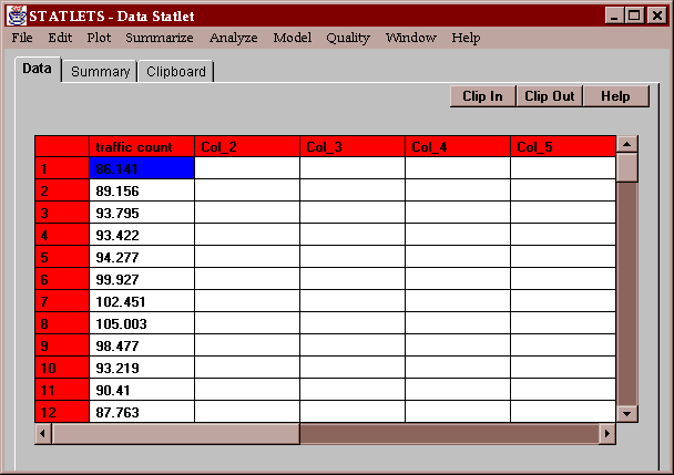
The example data consists of traffic counts on the Golden Bridge in San Francisco for each month from January, 1971 through December, 1978:

To use this statlet, you must specify the name of a single column of numeric data:
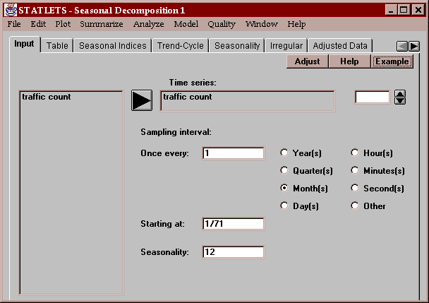
You must also enter additional information about the data, including:
Sampling interval - the interval between consecutive observations, such as once every year.
Starting at - the time period corresponding to the data value in the first row. Valid formats are:
year: a number such as 1901
quarter: a quarter such as Q1/95 indicating the first quarter of 1995.
month: an entry such as 06/85 representing June of 1985. The general format is mm/yy for month and year, where the two-digit years range from 1950 through 2049.
month: an entry such as 05/02/95 representing May 2, 1995. The general format is mm/dd/yy for month, day and year, where the two-digit years range from 1950 through 2049.
hour: a number such as 3 representing hour number 3.
minute: an entry such as 3:21 representing 3:21 a.m. Time is entered on a 24-hour scale.
second: an entry such as 13:25:30 representing 1:25:30 p.m. Time is entered on a 24-hour scale.
other: a number such as 1.
Seasonality - the periodicity of the data, such as 12 for monthly data that cycles once a year.
This tab displays the results of the seasonal decomposition:
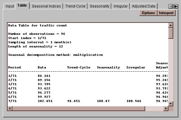
Each of the components of the decomposition is listed. The general approach to a decomposition follows several steps:
1. Smooth the data using a moving average of length equal to the length of seasonality. For example, a moving average of length 12 would be applied to monthly data. This estimates the trend-cycle.
2. Divide the data by the moving average (if using the multiplicative method) or subtract the moving average from the data (if using the additive method). This estimates the seasonality.
3. Average the results for each season separately and rescale so that an average month equals 100 (multiplicative) or 0 (additive). This gives the seasonal indices.
4. Adjust the data for the estimated trend-cycle and seasonality, yielding the irregular or residual component.
5. Divide the original data values by the appropriate seasonal index if using the multiplicative method, or subtract the index if using the additive method. This gives the seasonally adjusted data.
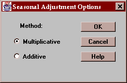
Select the desired method:
This tab shows the seasonal indices:
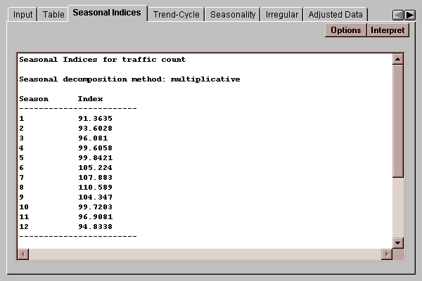
For the multiplicative method, the indices average 100. For the additive method, the indices average 0.
In this example, the index of 110.6 for month 8 indicates that traffic in August tends to average slightly more than 10% above that of an average month.
Select the desired method:

This tab shows the estimated trend-cycle:
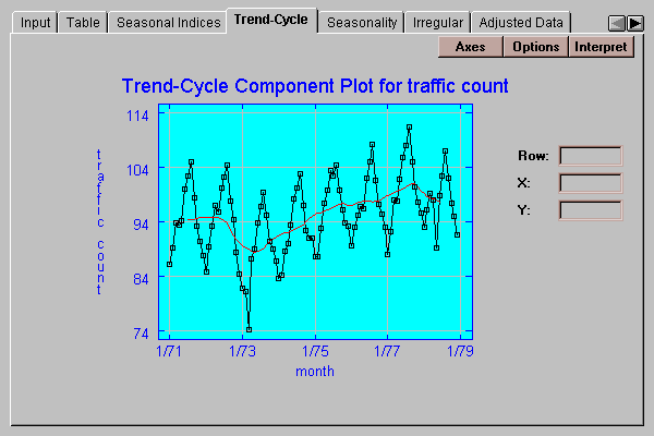
The solid line shows a moving average of length equal to the length of seasonality.
Select the desired method:

This tab plots the estimated seasonal indices:
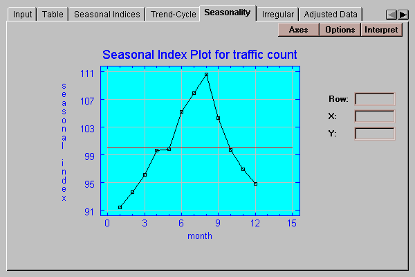
For the multiplicative method, the indices average 100. For the additive method, the indices average 0.
Select the desired method:

This tab shows the irregular or residual component:
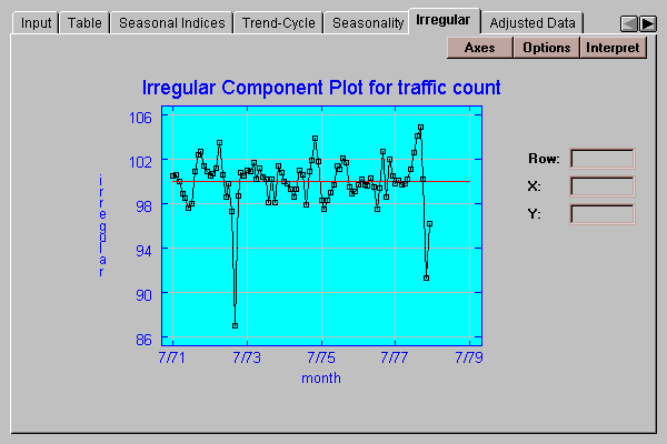
For the multiplicative method, the irregular component is rescaled to average 100. For the additive method, the component is rescaled to average 0.
Select the desired method:

This tab plots the seasonally adjusted data:
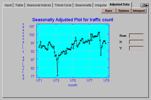
The seasonally adjusted data is the data with the estimated seasonal effects removed.
Select the desired method:

This tab displays a seasonal subseries plot:
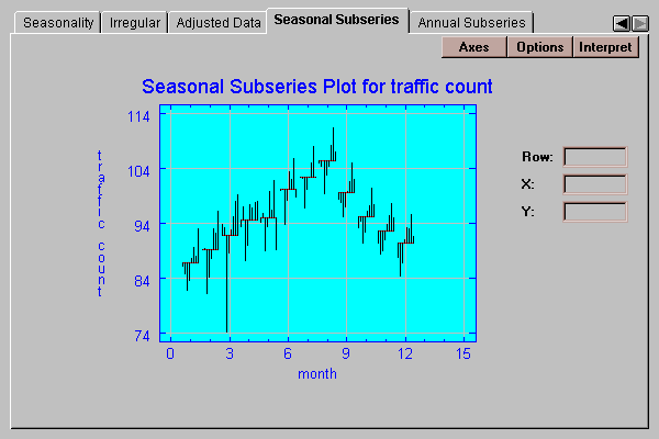
In this plot, the average for each month from January through December is plotted as a short horizontal line. Vertical lines are then drawn from each January to the average January, from each February to the average February, and so on. The seasonal component is readily seen by comparing the averages of the 12 months. Within each month, you can see the trend-cycle, while the length of the vertical lines represents the random component.
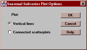
The plot may be drawn with vertical lines (as shown above) or with connections between the points within each season:
This tab displays an annual subseries plot:
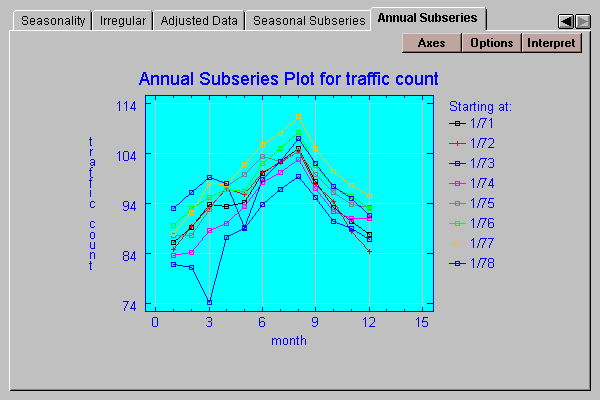
In this plot, the traffic volumes from each year are plotted separately for the 12 months.
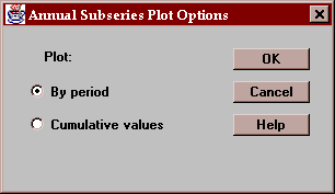
The points on the plot are the individual data values or the cumulative sums within each year:
