This statlet fits models relating a dependent variable Y to a single independent variable X. It fits a linear model of the form
Y = a + bX + e
and other nonlinear models which may transformed to the above form by transforming X, Y, or both. The method of least squares is used to estimate the intercept a and the slope b. The deviations around the regression line e are assumed to be normally and independently distributed with a mean of 0 and a standard deviation sigma which does not depend on X.
The statlet is the same as the Simple Regression statlet, except for the Predictions tab which generates predictions for X given Y instead of for Y given X.
The tabs are:
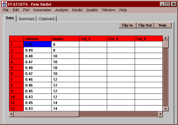
The example data shows the results of studies on the amount of chlorine available in a product as a function of the length of time since the product was produced. A total of 44 cartons were tested at ages ranging from 8 weeks to 42 weeks after production:
Enter the name of the column containing values of the dependent variable (Y) and the independent variable (X):
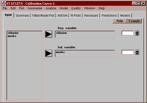
You may use the spinners to transform either or both of the variables.
This tab shows the results of fitting the currently selected model:
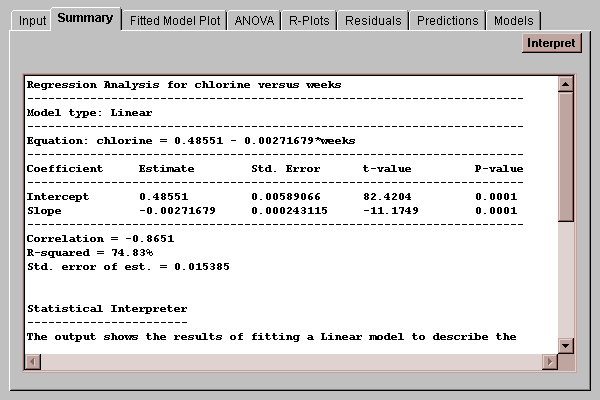
By default, a linear model is fit, although this may be changed by selecting the Models tab and pressing the Options button.
Of particular interest in the table are:
Estimate - this column shows the estimates of each of the unknown parameters in the model. The fitted model is
Chlorine = 0.48551 - 0.00271679*weeks
Std. Error - this column shows the estimated standard errors of the intercept and slope. The standard errors measure the estimation error in the coefficients and are used to test hypotheses concerning the intercept and slope.
t-value - this column shows t statistics, computed as
t = estimate / standard error
which can be used to test whether or not the intercept and slope are significantly different from zero.
P-value - the results of hypothesis tests of the form
- H0: intercept equal 0
- HA: intercept not equal 0
and
- H0: slope equal 0
- HA: slope not equal 0
The P-value gives the probability of getting a value of t with absolute value greater than that observed if the null hypothesis H0 is true. If the P-value falls below 0.05, then we reject the null hypothesis at the 5% significance level. We could then assert that we are 95% confident that the true parameter is not zero.
In the case of the chlorine data, note that both P-values are well below 0.05 (even below 0.01). We can therefore be very confident that neither the intercept nor the slope equals 0. Of the two hypothesis tests, the test concerning the slope is of more interest, since a slope equal to 0.0 would imply that weeks had no relationship to chlorine. By rejecting the hypothesis that the slope equals 0.0, we assert a statistically significant relationship between chlorine and the number of weeks since production. (Note: the hypothesis of zero slope could also be tested using the ANOVA table. In simple regression, the P-value in that table will always be identical to the P-value for the t test concerning the slope).
To summarize the usefulness of the model, a number of other statistics are also displayed. The first statistic is the correlation coefficient r. This coefficient ranges between -1 and 1 and measures the strength of the linear relationship between Y and X. The value of -0.865 indicates a moderately strong negative correlation between chlorine and weeks (Y goes down as X goes up).
The second statistic, R-squared, is called the coefficient of determination and measures the percent of the variability in Y which has been explained by the model. For the chlorine data, R-squared equals 74.8%, which indicates that the fitted model explains almost three-fourths of the variability in the 44 measured chlorine values. The remaining 25% must be due to other factors, such as measurement error, natural variability in the raw materials used to make the product, or failure of the straight line model to capture the true relationship between chlorine and weeks.
A third statistic, called the standard error of the estimate, estimates the standard deviation of the noise or deviations around the fitted model. The current estimate of 0.0154 is be used by the Predictions tab to form confidence limits for the line and predictions limits for new observations.
This tab shows a plot of the fitted model:
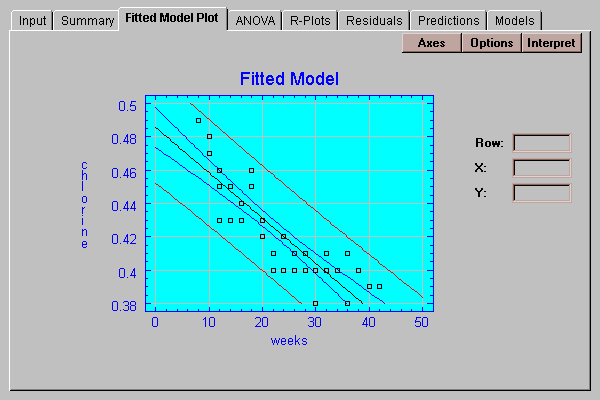
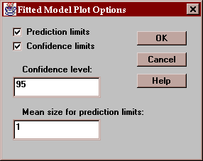
Also displayed are two sets of limits:
Prediction limits for the average of k new observations taken at a specific value of X (outer limits). By default, k=1, so the limits apply to single additional observations. When drawn at the default level of 95% confidence, they indicate the region in which we expect 95% of any additional observations to lie.
Confidence limits for the mean of many new observations taken at a specific value of X (inner limits). These limits display how well the location of the line has been estimated given the current sample size.
Use the Options button to specify the type of limits to be displayed and the confidence level for those limits:
This tab displays an analysis of variance table:
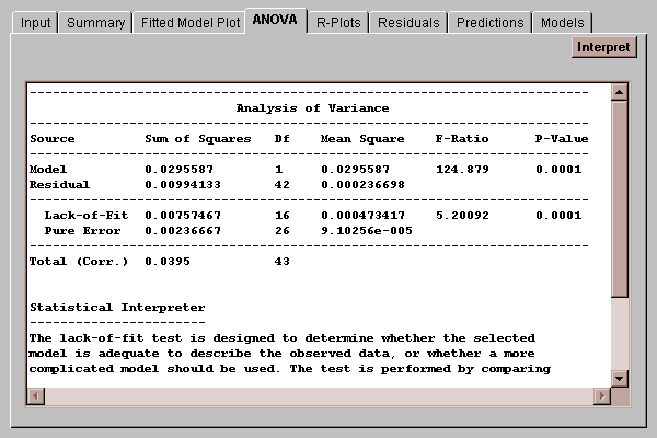
The ANOVA table divides the total variability in Y into two pieces: one piece due to the model, and one piece left in the residuals, such that
Total Corrected SSQ = Model SSQ + Residual SSQ
where SSQ stands for "Sum of Squares". The R-squared statistic displayed by the Summary tab is the ratio
R-squared = Model SSQ / Total Corrected SSQ
If the data contains replicate measurements (more than one data value at the same X), the table will also display the result of a lack-of-fit test run to determine whether the straight line adequately describes the relationship between Y and X. It decomposes the residual sum of squares into two pieces:
Residual SSQ = Lack-of-fit SSQ + Pure Error SSQ
In essence, what is happening is that the variability of the residuals around the fitted line is being divided into two pieces:
The table shows the results of an F test comparing the estimated lack-of-fit to pure error through
F = Lack-of-Fit Mean Square / Pure Error Mean Square
Of primary interest is the P-value associated with the test. Small values of P (less than 0.05) indicate significant lack-of-fit at the 5% significance level. For the chlorine example, the F-statistic equals 5.2 with a P-value well below 0.01. This indicates that the straight line does not give an adequate representation of the true relationship between chlorine and weeks. In such a case, you should select the Models tab which fits other curvilinear models.
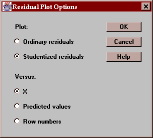
This tab plots the residuals from the fitted model versus values of X:
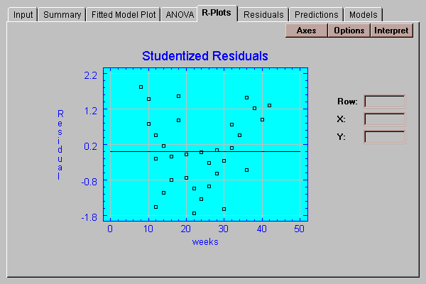
By definition, the residuals are equal to the observed data values minus the values predicted by the fitted model. You may plot either:
Ordinary residuals - in units of the dependent variable.
Studentized residuals - in units of standard deviations.
The Studentized residual equals
Studentized residual = residual / sresidual
where sresidual is the estimated standard error of the residual when the line is fit using all data values except the one for which the residual is being computed. These "Studentized deleted residuals" therefore measure how many standard deviations each point is away from the line when the line is fit without that point. In moderately sized data sets, Studentized residuals of 3.0 or greater in absolute value may well indicate outliers which should be treated separately.
Notice that between 20 and 30 weeks, virtually all of the residuals are less than 0.0, indicating that the data points fall below the fitted line. At extremely low and high values of weeks, the residuals are predominantly positive. Such residual plots are extremely valuable at illustrating curvature, especially when fitting models involving several independent variables.
Enter the type of residuals to be plotted and what they should be plotted against:
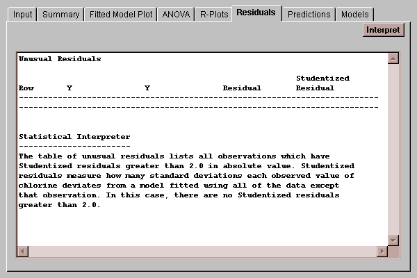
This table shows any Studentized residual in excess of 2.0 in absolute value:
The Studentized residual equals
Studentized residual = residual / sresidual
where sresidual is the estimated standard error of the residual when the line is fit using all data values except the one for which the residual is being computed. These "Studentized deleted residuals" therefore measure how many standard deviations each point is away from the line when the line is fit without that point. In moderately sized data sets, Studentized residuals of 3.0 or greater in absolute value may well indicate outliers which should be treated separately.
This tab creates a table of predicted values for the independent variable:
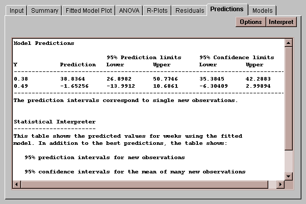
Each prediction is shown with two sets of limits, corresponding to the type of limits displayed on the Fitted Model Plot:
Prediction limits for X given the average of k new values of Y. By default, k=1, so the limits apply to X given a single additional observation on Y.
Confidence limits for X given the mean of many new observations.
Use the Options button on the Fitted Model Plot tab to modify the default selections.
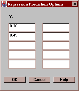
Select up to 10 values of Y at which predictions are to be made:
This table shows the results of fitting 12 different types of models to the data:
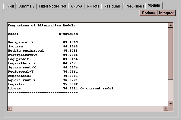
The models are listed in decreasing order of R-squared. Each of the models can be made linear by transforming either Y, X, or both and is called a "transformable nonlinear model". For example, the multiplicative model is defined by
Y = aebX
It can be linearized by taking natural logarithms of both sides, giving
ln(Y) = a* + bX
where a*=ln(a). Models near the top of the list may be good alternatives if the linear model is not adequate for the data.
Select the primary model to fit to the data:
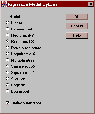
The model selected here becomes the model displayed in all of the other tabs. For example, choosing a reciprocal-X model for the example data shows the following Fitted Model Plot:
