This statlet estimates a wide variety of statistical models which may be used to forecast future values of a time series. The models include a random walk, different types of trends, moving averages, seasonal and nonseasonal exponential smoothers, and univariate ARIMA models. Confidence limits are calculated for all forecasts.
The tabs are:
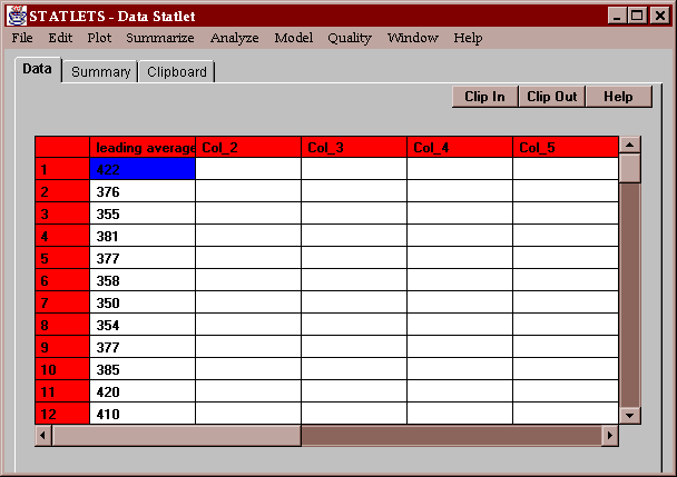
The example data consists of the leading batting average in U.S. major league baseball for every year from 1901 to 1995:

To use this statlet, you must specify the name of a single column of numeric data:
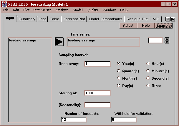
You must also enter additional information about the data, including:
Sampling interval - the interval between consecutive observations, such as once every year.
Starting at - the time period corresponding to the data value in the first row. Valid formats are:
year: a number such as 1901
quarter: a quarter such as Q1/95 indicating the first quarter of 1995.
month: an entry such as 06/85 representing June of 1985. The general format is mm/yy for month and year, where the two-digit years range from 1950 through 2049.
month: an entry such as 05/02/95 representing May 2, 1995. The general format is mm/dd/yy for month, day and year, where the two-digit years range from 1950 through 2049.
hour: a number such as 3 representing hour number 3.
minute: an entry such as 3:21 representing 3:21 a.m. Time is entered on a 24-hour scale.
second: an entry such as 13:25:30 representing 1:25:30 p.m. Time is entered on a 24-hour scale.
other: a number such as 1.
(Seasonality) - optional entry indicating the periodicity of the data, such as 12 for monthly data that cycles once a year.
Number of forecasts - the number of periods beyond the end of the data at which forecasts are desired.
Withhold for validation - the number of periods at the end of the data which will be withheld for validation. If greater than 0, these periods will not be used to fit the forecasting model. However, separate summary statistics on forecasting performance will be calculated for these periods.
This tab displays the forecasts generated by the currently selected forecasting model:
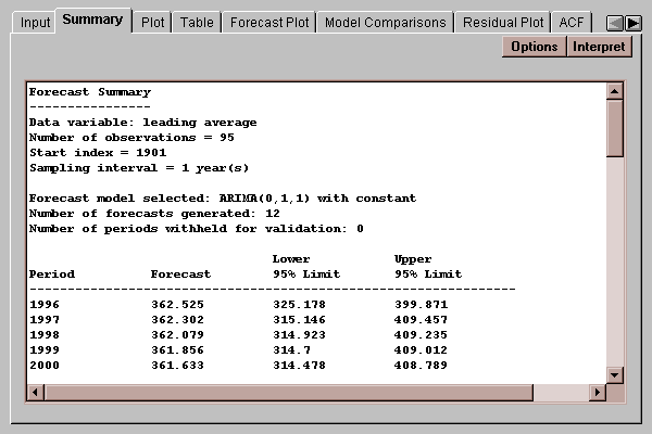
By default, the statlet uses an ARIMA model of order (0,1,1) with a constant for nonseasonal data and a (0,1,1)x(0,1,1) Arima model with a constant for seasonal data. This may be changed by pressing the Options button. To compare different forecasting models, press the Model Comparisons tab.
The table shows the forecasts for the periods immediately the last data value, together with 95% forecast limits. The forecasts show the best guess for the time series, projecting past behavior into the future. The forecast limits provide intervals in which we have 95% confidence that the true values will fall, assuming that we have selected an appropriate model and assuming that the future behaves in a similar manner to the past. To the extent that the data used to build the model are consistent with future behavior, these limits should be accurate.
The second half of the summary shows error statistics for the selected model:
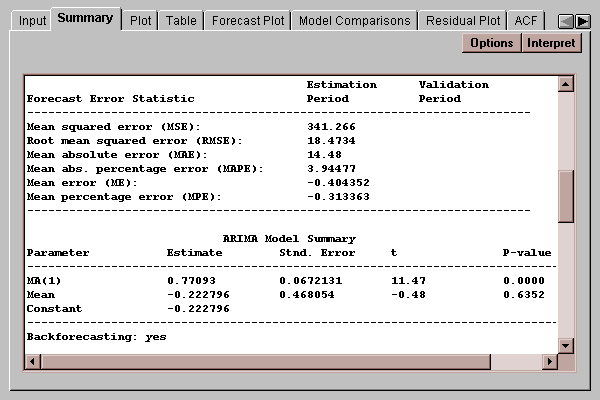
The statistics displayed are calculated from the one-ahead forecast errors. This is the difference between the actual data value at time t and the forecast that would have been made for that period given the data through time t-1. Included are the:
MSE - the average or mean of the squared errors.
RMSE - the square root of the MSE.
MAE - the mean of the absolute values of the one-ahead errors.
MAPE - the mean of the absolute values of the errors, as a percentage of the actual values. This is only calculated if all data values are greater than 0.
ME - the average or mean of the errors.
MPE - the mean error as a percentage of the actual values. This is only calculated if all data values are greater than 0.
The MSE, RMSE, MAE, and MAPE measure the magnitude of the forecast errors. Better models will show smaller values for these statistics. The ME and MPE are measures of bias. Better models will show values closer to 0. The above model errs in predicting the following year's batting average by approximately 14 points or 4% on average.
If the input panel requested that a certain percentage of the data be withheld for validation, separate statistics will be displayed for the time periods used to fit the model and the validation period. If the statistics in the two periods are similar, we would have increased confidence that the model will give good forecasts for the future.
For certain models such as the ARIMA model, the table also displays summaries of the estimated coefficients. In this case, the fitted model is
(Yt-Yt-1) = -0.222796 + at - 0.77093*at-1
or
Yt = Yt-1 - 0.222796 + at - 0.77093*at-1
where at represents a random shock or error added to the system at time t. The P-values indicate that the MA(1) coefficient is significantly different from 0, although the constant term is not.
Use this button to select the forecasting model to be used:

The available models are:
Random walk - this model assumes that the time series is equally likely to go up or down from its present position at time t. Consequently, the best forecast at time t for the value of the time series at time t+k is the value of the series at time t, i.e.,
Ft+k = Yt
Constant mean - this model assumes that the data vary randomly around a fixed mean. The best forecast for time t+k is the average of all previous values, i.e.,
Ft+k = average of (Y1, Y2, ..., Yt)
Linear trend - this model assumes that the data vary randomly around a straight line with intercept a and slope b. The best forecast for time t+k is an extrapolation of the least squares line fit to the data from periods 1 through t, i.e.,
Ft+k = a + b*(t+k)
where a and b are the estimated intercept and slope, respectively.
Quadratic trend - this model assumes that the data vary randomly around a quadratic regression line. The best forecast for time t+k is an extrapolation of the least squares line fit to the data from periods 1 through t, i.e.,
Ft+k = a + b*(t+k) + c*(t+k)2
Exponential trend - this model assumes that the data vary randomly around an exponential regression line. The best forecast for time t+k is an extrapolation of the least squares line fit to the data from periods 1 through t, i.e.,
Ft+k = exp(a + b*(t+k))
S-curve trend - this model assumes that the data vary randomly around an S-curve regression line. The best forecast for time t+k is an extrapolation of the least squares line fit to the data from periods 1 through t, i.e.,
Ft+k = exp(a + b/(t+k))
Simple moving average - this model forecasts future data by taking the average of the last m values. Indicate the number of terms m, which by default is 5, so that
Ft+k = (Yt-4 + Yt-3 + Yt-2 + Yt-1 + Yt) / 5
Simple exponential smoothing - this model forecasts future values by taking a weighted average of all previous data values, where more weight is given to recent observations than to older observations. The forecast for time t+k is given by
Ft+k = alphaYt + alpha(1-alpha)Yt-1 + alpha(1-alpha)2Yt-2 + alpha(1-alpha)3Yt-3 + ...
where alpha is a called the smoothing constant and must lie between 0 and 1. The closer alpha is to 0, the more weight is given to older observations. As alpha tends to 0, the model approaches the simple mean model. As alpha tends to 1, the model approaches a random walk. By default, STATLETS selects whatever value of alpha minimizes the mean squared error (MSE). You can fix the value of alpha by removing the check for the "optimize" checkbox.
Brown's linear exponential smoothing - this model forecasts future values by estimating and extrapolating a linear trend. The intercept and slope are based on weighted averages of all previous data values, controlled by a single smoothing constant alpha.
Brown's quadratic exponential smoothing - this model forecasts future values by estimating and extrapolating a quadratic trend. The model coefficients are based on weighted averages of all previous data values, controlled by a single smoothing constant alpha.
Holt's linear exponential smoothing - this model forecasts future values by estimating and extrapolating a linear trend. The intercept and slope are based on weighted averages of all previous data values, using separate smoothing constants for the intercept and slope.
Winter's seasonal exponential smoothing - only available for seasonal data, this model forecasts future values by estimating and extrapolating a linear trend, adjusting the data in each season by estimated seasonal indices. The intercept, slope, and seasonal indices are based on weighted averages of all previous data values, using separate smoothing constants for each.
ARIMA models - autoregressive, integrated, moving average models which express the data value at time t as a linear combination of previous data values and/or current and previous random shocks to the system. Specify:
p = order of autoregressive part of the model
d = order of differencing
q = order of moving average part of the model
constant = whether or not a constant should be included in the model
For seasonal data, separate values of p, d and q are requested for the nonseasonal and seasonal parts of the model.
This tab shows a plot of the data and forecasts:
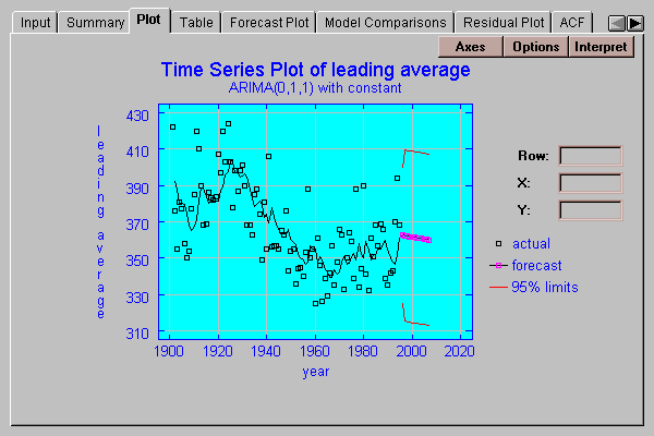
It shows:
actual data values - the small black squares are the data used to fit the model.
forecasts - the line shows the one-ahead forecasts over the period containing the data, and the forecasts made from the end of the data for the next several periods.
95% limits - the 95% forecast limits.
Specify the confidence level for the forecast limits:
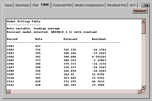
This tab displays the data used to fit the model, the one-ahead forecasts, and the residuals:
This tab shows a plot of the last several data values and the forecasts:
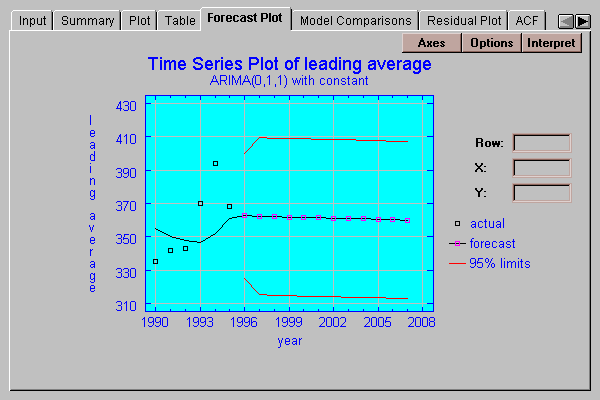
It shows:
actual data values - the small black squares are the data used to fit the model.
forecasts - the line shows the one-ahead forecasts over the period containing the data, and the forecasts made from the end of the data for the next several periods.
95% limits - the 95% forecast limits.
Specify the confidence level for the forecast limits:

This tab displays a comparison of several different forecasting models when fit to the data:
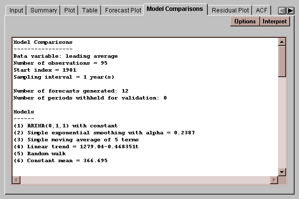
The top half of the table lists the models. Six models are fit by default. You can select others by pressing the Options button.
The bottom half of the table shows a comparison of the models:
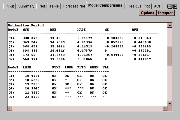
Each model is shown together with summary statistics as discussed in the Summary tab. Notice that model (1), the ARIMA(0,1,1) model, gives the smallest MSE, MAE, and MAPE. These statistics are often used to compare competing models.
The bottom section of the table shows the results of applying a number of tests to the residuals to determine whether they are random, as they should be if a model fits the data adequately. Five tests are performed:
RUNS - counts the number of runs up and down
RUNM - counts the number of runs above and below the median
AUTO - performs a Box-Pierce test on the residual autocorrelations
MEAN - compares the mean of the first half of the residuals to the mean of the second half
VAR - compares the variance of the first half of the residuals to the variance of the second half
The first three tests are discussed in detail in the Randomness Tests section.
An indication is given as to how well each model performed:
OK - test was not significant at the 10% level or lower
* - test was significant at the 10% level
** - test was significant at the 5% level
*** - test was significant at the 1% level
A model such as model (6), which shows highly significant test results on several tests, evidently fails to capture the dynamic structure of the data. A model such as model (1), which passes all of the tests, would be a good choice.
To select a different model than is currently fit to the data, return to the Summary tab and press the Options button. All of the other tabs will be updated to reflect the change.
Select each of the forecasting models to be compared:
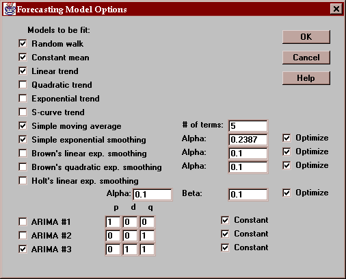
For a description of each model, refer to the Summary tab.
This tab plots the residuals:
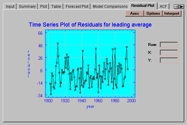
The residuals are equal to the one-ahead forecast errors, i.e., the difference between the observed value at time t and the forecast which would have been made for that time period given all of the information up to and including time period t-1.
Select either a scatterplot of the residuals or a normal probability plot:
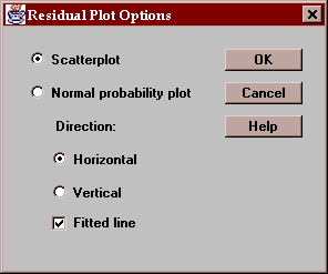
The normal probability plot is used to determine whether the residuals come from a normal distribution.
This tab creates a table displaying the residual autocorrelation coefficients:
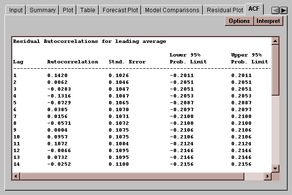
The autocorrelation at lag k
rk = corr(residualt, residualt-k)
varies between -1 and +1 and measures the correlation between residuals k time periods apart. If the residuals are random, the autocorrelation at all lags should be close to 0.
The table shows the autocorrelations for lags 1 through the value specified using the Options button. It also displays the large lag standard error for each coefficient, which estimates the standard error for rk assuming that all correlations at lag k and higher lags equal 0. This standard error is used to derive the probability limits in the two rightmost columns of the table. Any autocorrelation outside the 95% probability limits is significantly different from zero at the 5% significance level.
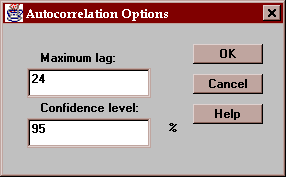
Specify the maximum lag to be included on the table and the confidence level for the probability intervals:
This tab plots the sample autocorrelation coefficients with probability limits:
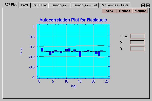
The height of each bar shows the magnitude of the autocorrelation at a selected lag. The red lines are 95% probability limits centered at 0. An estimate outside the limits would allow us to reject the hypothesis that the autocorrelation at that lag is equal to 0. In this case, the autocorrelations are all within the 95% limits. This is typical of a random set of residuals.
Specify the maximum lag to be included on the table and the confidence level for the probability intervals:

This tab creates a table displaying the residual partial autocorrelation coefficients:
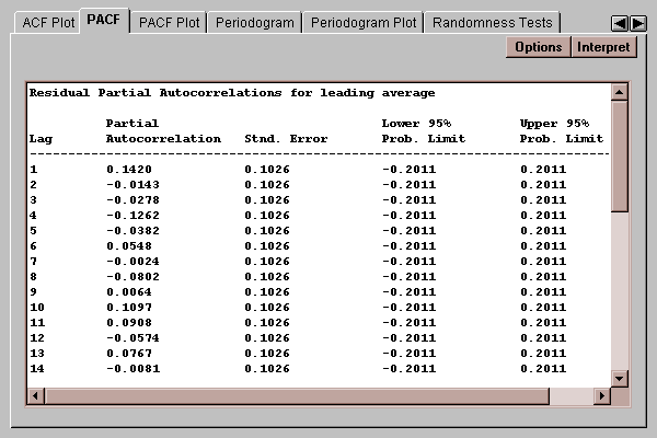
The partial autocorrelation at lag k measures the correlation between residuals separated by k time units, accounting for any correlation at lower lags. The partial autocorrelations are shown together with their standard errors, which are in turn used to calculate the probability limits. Any partial autocorrelation outside the 95% probability limits is significantly different from zero at the 5% significance level.
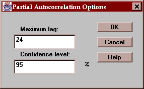
Specify the maximum lag to be included on the table and the confidence level for the probability intervals:
This tab plots the residual partial autocorrelation coefficients with probability limits:
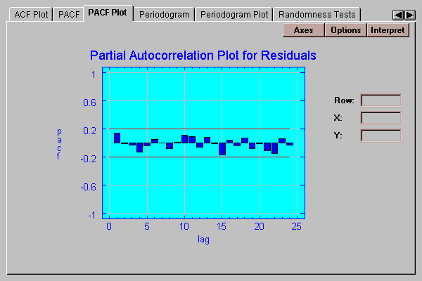
The height of each bar shows the magnitude of the partial autocorrelation at a selected lag. The red lines are 95% probability limits centered at 0. An estimate outside the limits would lead us to reject the hypothesis that the partial autocorrelation at that lag is equal to 0.
Specify the maximum lag to be included on the table and the confidence level for the probability intervals:

This tab displays the residual periodogram and cumulative (integrated) periodogram:
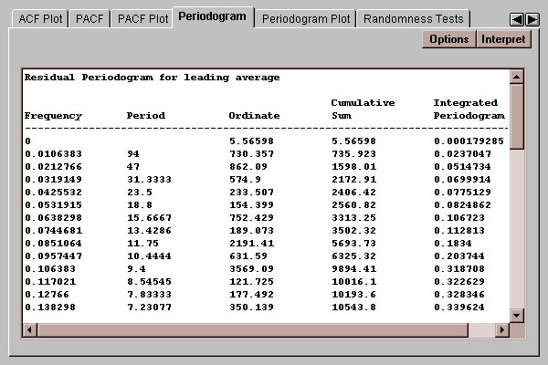
When the time series of interest has periodic components in it, i.e., fluctuations which repeat at regular frequencies, it can be instructive to express the time series as a sum of sines and cosines with different frequencies. It is well-known that any time series can be expressed as the sum of n/2 sine waves at frequencies corresponding to one cycle over the sampling period, two cycles, three cycles, and so on (called the Fourier frequencies). If the time series is random, the periodogram will be constant at all frequencies (to within normal sampling error). If it contains a strong trend, the low frequency terms will dominate.
The periodogram actually performs an analysis of variance by frequency. Summing the periodogram ordinates yields the total corrected sum of squares ordinarily displayed in an ANOVA table. In the above table, the rightmost column displays the cumulative sum of the ordinates divided by that total. It is used to help determine whether the residual time series is random in the Integrated Periodogram plot.
Specify options for periodogram:
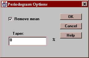
Remove mean - if checked, the sample mean is first subtracted from the data before the periodogram ordinates are computed. If this is not done, a large spike at lag 0 normally results.
Taper - if desired, a cosine-bell taper may be used to adjust a given percentage of the values at both ends of the time series. This is sometimes done to reduce end effects.
This tab displays a plot of the residual periodogram:
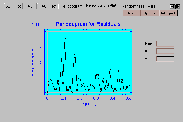
The periodogram is described in the previous section. In this case, the periodogram is fairly uniform over all frequencies..
Specify options for periodogram:

Remove mean - if checked, the sample mean is first subtracted from the data before the periodogram ordinates are computed. If this is not done, a large spike at lag 0 normally results.
Taper - if desired, a cosine-bell taper may be used to adjust a given percentage of the values at both ends of the time series. This is sometimes done to reduce end effects.
This tab shows the results of three tests used to determine whether or not the residuals are random:
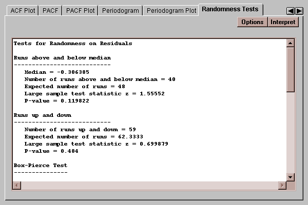
A random time series is a sequence of random numbers with no inherent dynamic structure or autocorrelation. If our forecasting model has captured all of the dynamic structure in the data, the residuals should form a random sequence of numbers.
Three tests are performed:
Runs above and below median - counts the number of times that the residual time series rises above or below the sample median and compares that to the value expected for a random sequence of numbers.
Runs up and down- counts the number of times that the residual time series rises or falls and compares that to the value expected for a random sequence of numbers.
Box-Pierce test - calculates the first k lagged autocorrelations and calculates a statistic which follows a chi-squared distribution.
Each test calculates a P-value. A P-value below 0.05 would lead us to reject the hypothesis that the residuals are random at the 5% significance level.
In this case, all P-values are well above 0.05.
Specify the number of terms to be used in the Box-Pierce test:
This tab plots the integrated periodogram:
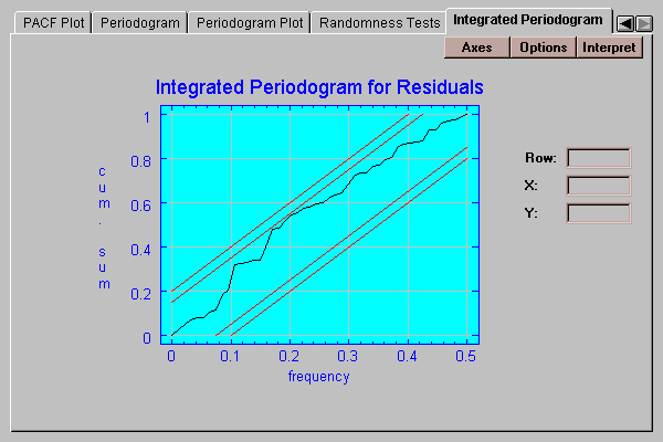
Included on the plot are 90% and 95% Kolmogorov-Smirnov bounds. If the plotted function remains within those bounds, which it does in this case, we cannot reject the hypothesis that the residuals time series is random at the 10% and 5% significance levels, respectively.
Specify options for periodogram:

Remove mean - if checked, the sample mean is first subtracted from the data before the periodogram ordinates are computed. If this is not done, a large spike at lag 0 normally results.
Taper - if desired, a cosine-bell taper may be used to adjust a given percentage of the values at both ends of the time series. This is sometimes done to reduce end effects.