This statlet fits models relating a dependent variable Y to one or more independent variables. It fits a model of the form
Y = a + bX1 + cX2 + dX3 + ... + e
The method of least squares is used to estimate the model coefficients. The deviations around the regression line e are assumed to be normally and independently distributed with a mean of 0 and a standard deviation sigma which does not depend upon the levels of the independent variables.
The tabs are:
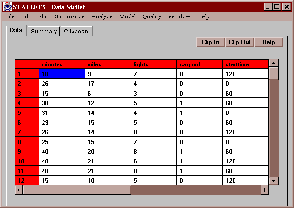
The example data contains information on the commuting times of 25 students at a local community college. The data include each student's commuting time in minutes, the number of miles traveled, the number of traffic lights passed, whether or not the student is part of a carpool (0=no, 1=yes), and the starting time of the student's first class in minutes after 8:00 AM:

Enter the names of the columns containing values of the dependent variable (Y) and the independent variables (X1-Xk):
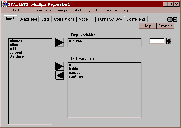
You may use the spinner to transform the dependent variable.
This tab displays a scatterplot matrix for the variables in the analysis:
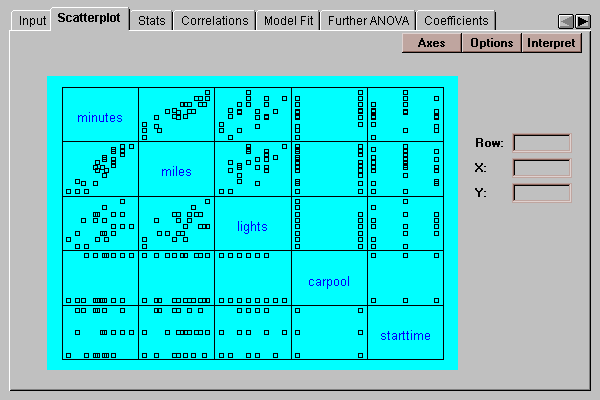
The matrix consists of a set of two-variable scatterplots, where a selected variable such as "minutes" forms the Y-axis of all plots in its row and the X-axis of all plots in its column. This plot is useful for:
Clicking on a point in any plot causes that point to be highlighted in all of the plots.
The Option button allows you to smooth the two-variable scatterplots using any of four different methods:
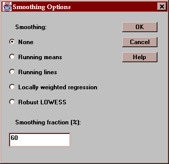
The different smoothing methods are described in the Y versus X Scatterplot statlet. The plot below shows the result of selecting "robust LOWESS" with the default smoothing fraction:

This tab displays summary statistics for each of the variables:
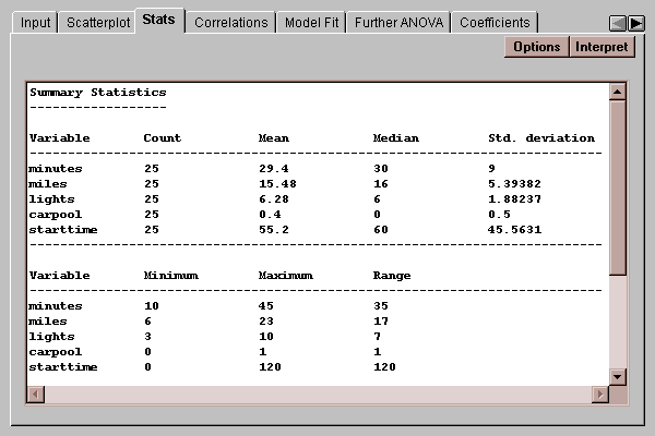
The statistics are calculated from all rows which have no missing values for any of the variables.
Select the statistics to be calculated:
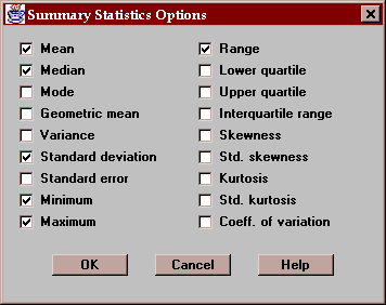
For a description of each of the statistics, see the Glossary.
This tab shows a table of Pearson product-moment correlations for the variables:
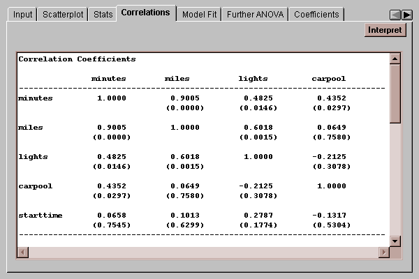
Correlations measure the strength of the linear relationship between two variables on a scale of -1 to +1. In parentheses below each correlation is a P-value which tests the hypotheses:
H0: correlation equal 0
HA: correlation not equal 0
Any P-value below 0.05 corresponds to a statistically significant correlation at the 5% significance level.
The correlations are calculated from all rows which have no missing values for any of the variables.
This tab shows the results of fitting the multiple regression model:
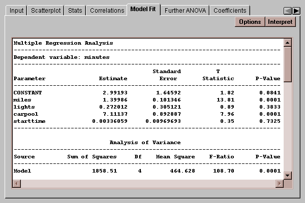
By default, a model is fit using all of the specified independent variables, although a stepwise regression may be requested by pressing the Options button.
Of particular interest in the table are:
Estimate - this column shows the estimates of each of the coefficients in the model. The fitted model is
minutes = 2.99 + 1.40*miles + 0.272*lights + 7.11*carpool + 0.00336*starttime
Std. Error - this column shows the estimated standard errors of each coefficient. The standard errors measure the estimation error in the coefficients and are used to test hypotheses concerning their true values.
t-value - this column shows t statistics, computed as
t = estimate / standard error
which can be used to test whether or not the coefficient is significantly different from zero.
P-value - the results of hypothesis tests of the form
- H0: coefficient equal 0
- HA: coefficient not equal 0
The P-value gives the probability of getting a value of t with absolute value greater than that observed if the null hypothesis H0 is true. If the P-value falls below 0.05, then we reject the null hypothesis at the 5% significance level. We could then assert that we are 95% confident that the true parameter is not zero.
In this case, the coefficients corresponding to miles and carpool are statistically significant, while those corresponding to lights and starttime are not.
Several other statistics have also been calculated:
R-squared, called the coefficient of determination, which measures the percent of the variability in Y which has been explained by the model. R-squared is defined by
R-squared = 100*(Model SSQ / Total Corrected SSQ)%
where SSQ represents the sum of squares attributable to a factor.
The adjusted R-squared, which adjusts the above statistic for the number of independent variables in the model according to
Adj. R-squared = 100*(1-[(n-1)/(n-p)]*Error SSQ / Total Corrected SSQ)%
where n is the number of observations and p is the number of estimated coefficients in the model. This is a better statistic to use when comparing models with different numbers of coefficients.
The standard error of the estimate, which estimates the standard deviation of the noise or deviations from the fitted model.
The mean absolute error (MAE), which is the average of the absolute values of the residuals (the average error in fitting the data points).
The Durbin-Watson statistic, which looks for autocorrelation in the residuals based upon their sequential order. If the data were recorded over time, this statistic could detect time trends which, if accounted for, could improve the fitted model. Unfortunately, there is no P-value associated with the Durbin-Watson statistic, and it must be compared to tables to determine how significant it is. As a rule of thumb, when the Durbin-Watson statistics falls below 1.4 or 1.5, one should plot the residuals versus row number to see if there is any noticeable correlation between residuals close together in time. For a perfectly random sequence, the Durbin-Watson statistic would equal 2.0.
Use this button to control various model-fitting options:
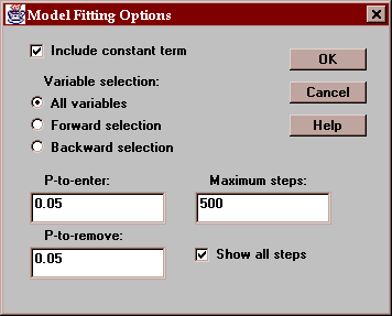
Include constant term - if checked, a constant term will be included in the regression model. Otherwise, the model will be forced through the origin.
Variable selection - select "All variables" to fit a model involving all of the independent variables. or select a stepwise regression procedure. Stepwise regression seeks to find a subset of the independent variables which provide a parsimonious yet significant description of the relationship amongst the variables.
Two methods of stepwise regression are provided:
Forward selection - variables are added to the model one at a time, in order of statistical significance, as long as the P-value of the next term to be added will be less than the "P-to-enter" specified on the dialog box.
Backward selection - beginning with a model involving all of the variables, variables are removed one at a time, the least significant first, as long as the P-value of the next term to be removed is greater than or equal to the "P-to-remove" specified on the dialog box.
In both cases, variables once entered may later be removed and vice versa if their contribution to the fitted model changes.
This tab shows the Type I Sums of Squares for each variable in the model:
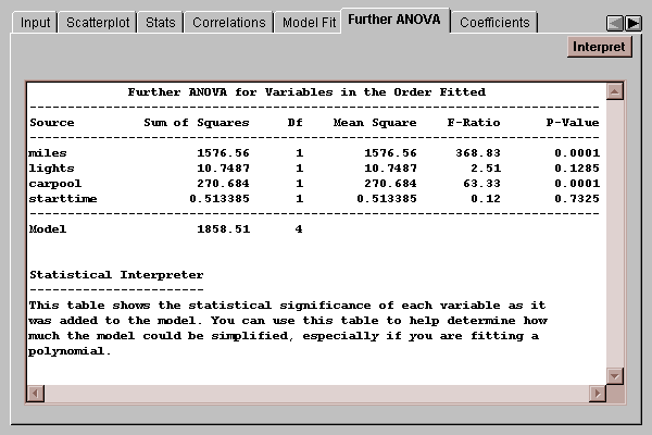
Type I sums of squares measure the contribution of a variable to the model sum of squares when added to the model in the order specified.
This tab shows confidence limits and variance inflation factors for each coefficient in the model, together with the correlation matrix for the estimated coefficients:
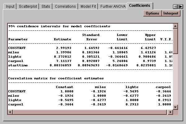
The variance inflation factors quantify the extent to which multicollinearity amongst the independent variables may be inflating their standard errors, making them less precise and difficult to interpret.VIF's in excess of 10 are usually seen as indicating a serious problem.
Enter the desired confidence level:
This tab displays a plot of the portion of the fitted model corresponding to a selected independent variable:
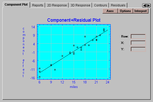
The solid line is defined by
component effect = coefficient * (X - Xbar)
where "coefficient" is the estimated coefficient of the selected independent variable and Xbar is the sample mean of that variable. The line passes through the point (Xbar,0) and has a slope equal to the coefficient of the independent variable. If you examine the change in Y indicated by the line between the lowest value of X and the highest value of X, you can get a sense of how large a swing in the dependent variable this independent variable represents. In the above plot, the line extends from -13 to +12, indicating that differences in miles traveled account for a swing of about 25 minutes in commuting times.
The points show the residuals added to the component effect. This lets you judge the relative importance of the selected independent variable in light of the noise in the data.
Select the independent variable for the plot:
The tab creates a report:
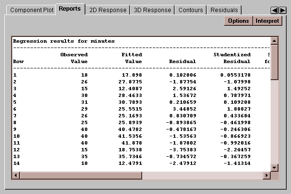
The report may contain various items, selected by pressing the Options button.
In the case of "Predicted Y", "Prediction limits", and "Confidence limits", a line is included in the table for all rows which have complete data for the X variables and a missing value for Y. To make predictions at different combinations of the X's, add additional rows to your file, entering data for the X variables but leaving the cells for the Y variable empty. This will not affect the fit but will affect this report.
Select the information to be displayed on the report:
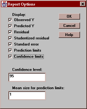
The last two entries correspond to:
Prediction limits for the average of k new observations taken at a specific value of X. By default, k=1, so the limits apply to single additional observations.
Confidence limits for the mean of many new observations taken at a specific value of the independent variables.
This tab displays a plot of the fitted model versus a selected independent variable, with all other variables held constant at the indicated values:
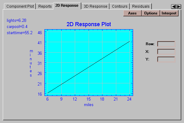
Select a variable to display along the X-axis and values at which to hold all of the other variables:
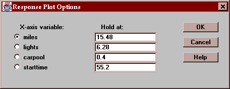
This tab displays a 3D surface plot of the fitted model versus 2 selected independent variables, with all other variables held constant at the indicated values:
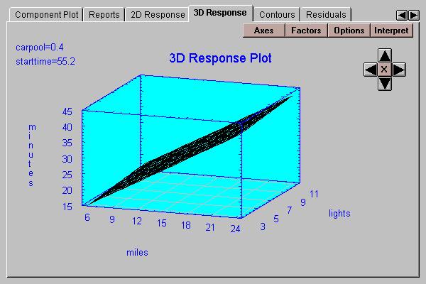
Select a variable to display along the X-axis, a variable to display along the Y-axis, and values at which to hold all of the other variables:

Specify the desired type of surface plot:
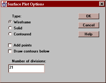
Enter:
Type - a wireframe plot for printing in black-and-white, a solid surface, or a surface made out of contour regions.
Add points - if checked, the data values will be included on the plot and lines will be drawn from each point to the surface.
Draw contours below - if checked, a contour plot will be drawn in the bottom plane of the cube. The contour levels will correspond to those selected on the Contours tab.
Number of divisions - determines how many lines will be drawn on the surface plot.
This tab displays a contour plot of the fitted model versus 2 selected independent variables, with all other variables held constant at the indicated values:
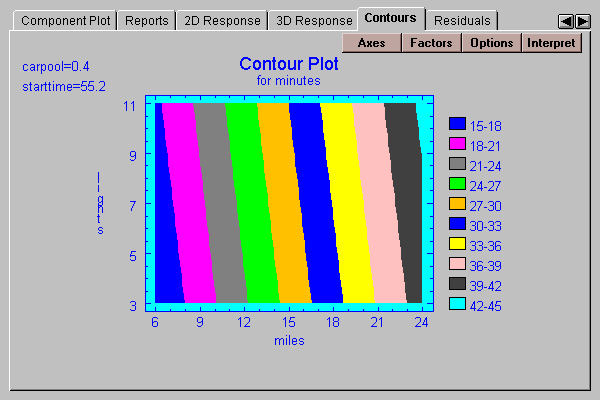
Each colored region corresponds to a predicted value for Y in the range indicated.
Select a variable to display along the X-axis, a variable to display along the Y-axis, and values at which to hold all of the other variables:

Select the type of contour plot:
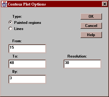
Enter:
Type - painted regions as shown above, or lines as on a topographical map.
From, to, by - defines the contours to be plotted.
Resolution - defines the resolution of the grid at which the function is evaluated. Higher resolutions give more accurate results but are more computationally expensive.
This table shows any Studentized residual in excess of 2.0 in absolute value:
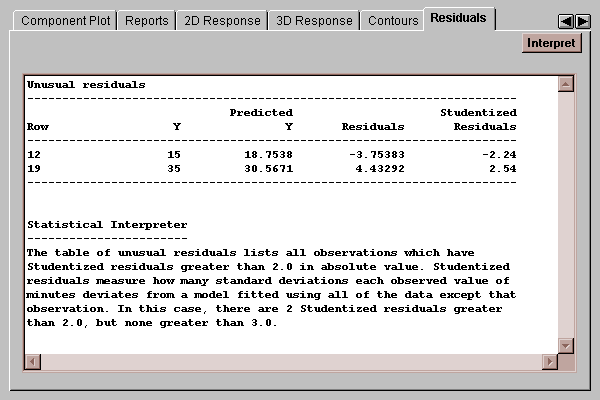
The Studentized residual equals
Studentized residual = residual / sresidual
where sresidual is the estimated standard error of the residual when the line is fit using all data values except the one for which the residual is being computed. These "Studentized deleted residuals" therefore measure how many standard deviations each point is away from the line when the line is fit without that point. In moderately sized data sets, Studentized residuals of 3.0 or greater in absolute value may well indicate outliers which should be treated separately.
This tab shows any data values which have an unusually large influence on the fitted model:
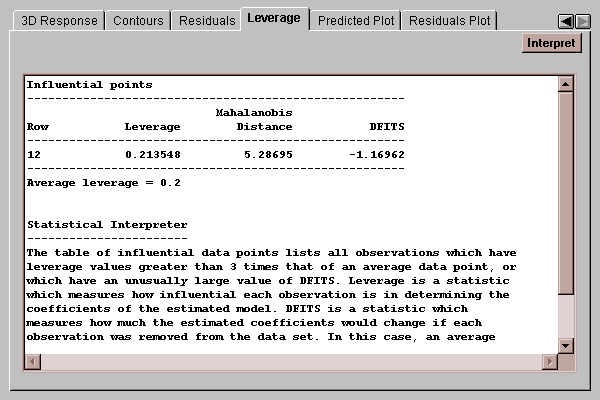
Three statistics are computed:
leverage - measures the relative influence of each data value on the model coefficients. Points with more than 3 times the average leverage are included on the list.
Mahalanobis distance - measures how far away from the centroid of the data each row lies in a multidimensional space defined by the independent variables.
DFITS - measures how much the estimated model coefficients would change if a row were removed from the fit. Rows with an unusually large value of DFITS are also shown on this list.
You should carefully examine any rows on this list to insure that they represent valid data, since they are especially influential in determining the fitted model.
This tab plots the observed values of Y versus the values predicted by the fitted model:
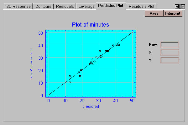
Any increase in scatter around the line as the predicted values increase could indicate the presence of heteroscedasticity, i.e., non-constant variability of the residuals.
This tab plots the residuals from the fitted model versus values of X:
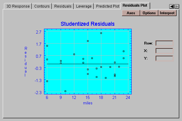
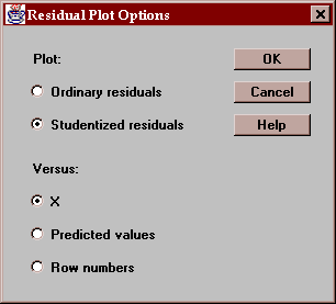
By definition, the residuals are equal to the observed data values minus the values predicted by the fitted model. You may plot either:
Ordinary residuals - in units of the dependent variable.
Studentized residuals - in units of standard deviations.
The Studentized residual equals
Studentized residual = residual / sresidual
where sresidual is the estimated standard error of the residual when the line is fit using all data values except the one for which the residual is being computed. These "Studentized deleted residuals" therefore measure how many standard deviations each point is away from the line when the line is fit without that point. In moderately sized data sets, Studentized residuals of 3.0 or greater in absolute value may well indicate outliers which should be treated separately.
Enter the type of residuals to be plotted and what they should be plotted against:
