 STATISTICAL COMPUTING ACTIVITY:
PRINCIPAL COMPONENT ANALYSIS FROM DATA
The data
set that we will be using is the 1988 Olympic Decathlon, given in Table 2.2.
Note that
Events: (1)
100m, (2) long jump, (3) shot putt, (4) high jump, (5) 400m, (6) 110m hurdles,
(7) discus, (8) pole vault, (9) javelin, (10) 1500m.
Step 1. Download olympic.xls from the web
site.
Step 2. Click on the file to open Excel
(We need to
modify the data first. That is the reason why we are running Excel.)
Step 3. Highlight the last row and delete it
by going Edit/Clear/All.
(Since this
athlete is a suspected outlier.)
Step 4. Transform the data by taking
negative values for the four running events, i.e., event1, event5, event6,
event10.
(So that
all events are scored in the same direction; small scores reflect poor
performance, large scores reflect the good performance.)
Step 5. Save the file as modoly.xls and
modoly.txt
Or
Step 1. Download modifiedolympic.txt from
the web site.
Step 2. Run R
Step 3. Go to File menu and ≥Change
directory≤ to the location that you have saved the file
>modoly=read.table(≥modifiedolympic.txt≤, header=T)
>attach(modoly)
To see the
variable names and data type
> modoly
Let us do
PCA by using correlation matrix
 STATISTICAL COMPUTING ACTIVITY:
PRINCIPAL COMPONENT ANALYSIS FROM A GIVEN COVARIANCE OR CORRELATION MATRIX
First we
need to learn how to enter a matrix
>example1=matrix(c(1,2,3,4,5,6), nrow=3, byrow=T)
To see the
matrix
>example1
Now try
>example2=matrix(c(1,2,3,4,5,6), nrow=2, byrow=T)
>example2
Now enter
the correlation matrix for the weekly rates of return for Allied Chemical,
duPont, Union Carbide, Exxon, and Texaco.

>return=matrix(c(1, .577, .509, ä , .523, 1), nrow=5,
byrow=T)
>eigen(return)
 STATISTICAL COMPUTING ACTIVITY:
PRINCIPAL COMPONENT ANALYSIS FROM DATA
Step 1. Download olympic.xls from the web
site.
Step 2. Run SYSTAT
File
Open
Data
Change Files of Type to All Files (*.*)
Locate the folder that you have saved the file
Select the file
Click Open
Click on line 34
Edit
Cut
To change
the signs of event1, event5, event6, event10
Data
Transform
=Let
Type negevent1 in the Variable box and -event1 in the Expression
box
Repeat this for event5, event6, and event10
Analysis
Multivariate
Analysis
Factor
Analysis
From Available variable(s) window select negevent1, event2,
event3, event4, negevent5, negevent6, event7, event8, event9, negevent10 by
double clicking on them
Make sure that Principal components (PCA) is selected as
Method and Correlation is selected as Matrix for extraction
Get rid off 1 and type 0 in the Minimum eigenvalue window.
Check extended results
Click on Save tab
Select Factor scores
Check Save data with scores
Click on ä at the end of the Filename and select where you
want to save the file
Type a file name, say olympicpca
Click OK
 STATISTICAL COMPUTING ACTIVITY:
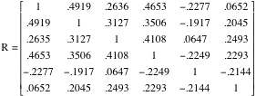
PRINCIPAL COMPONENT ANALYSIS FROM A GIVEN COVARIANCE OR CORRELATION MATRIX
Over a
period of five years, yearly samples of fishermen on 28 lakes in Minnesota were
asked to report the time they spent fishing and how many of each type of gane
fish they caught. Their responses were then converted to a catch rate per hour
for
x1=Bluegill,
x2=Black crappie, x3=Smallmouth bass, x4=Largemouth
bass, x5=Walleye, x6=Northern pike.
Fish caught
by the same fisherman live alongside of each other, so the data should provide
some evidence on how the fish group. The first four fish belong to the
centrarchids, the most plentiful family. The walleye is the most popular fish
to eat.
Now let us
carry out principal component analysis on this data

First we
need to enter correlation matrix to SYSTAT
Utilities
Matrix
Read
Give a name to your matrix, say fish
Since
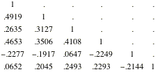
the matrix is symmetric it is enough to
enter diagonal and lower diagonal elements of the matrix remaining
values will be entered as ≥.≤:

On the keyboard data window you enter the matrix like
this
firstrow; secondrow; thirdrow ä (That is rows elements
are separated with commas, rows separated with semi colons. Here it is:
1, ., ., ., ., .; .49919, 1, ., ., ., .; .2635, .3127, 1,
., ., .; .4653, .3506, .4108, 1, ., .; ää..
Check column names and type variable names on
the window: say x1, x2, x3, x4, x5, x6
Check save matrix, by clicking on ä on
the next window select the folder that you would like to save the file and type
a name, say fishcor. Also select Correlation from the last window.
Click OK
Now we
will load the file
Edit
Open
Data
Locate the fishcor and double click.
Analysis
Multivariate
Analysis
Factor
Analysis
Perform a PCA using only x1 through x4.
Perform a PCA using all six variables.
Interpret your results.
![]() STATISTICAL COMPUTING ACTIVITY:
PRINCIPAL COMPONENT ANALYSIS FROM DATA
STATISTICAL COMPUTING ACTIVITY:
PRINCIPAL COMPONENT ANALYSIS FROM DATA

